GalMag basic tutorial
Welcome to the GalMag tutorial and basic usage guide.
Quick start
The code uses an object named B_field to store all the magnetic field information.
Associated with this, there is a coordinate grid which has to be set up at the time of the B_field initialization.
[1]:
import galmag
from galmag.B_field import B_field
import numpy as np
import matplotlib.pyplot as plt

# Maximum and minimum values of the coordinates for each direction
box_limits = [[-15, 15],[-15, 15],[-15, 15]] # kpc
box_resolution = [100,100,100]

B = B_field(box_limits, box_resolution)
The grid - which is an uniform cartesian grid in the default case - can be accessed through the attribute B_field.grid.
This attribute contains a Grid object, which itself contains numpy arrays in the coordinate attributes x, y, z, r_cylindrical, r_spherical, theta and phi.
The coordinate systems place the galactic mid-plane at \(z=0\), \(\theta = \pi/2\).
[2]:
# Example access to the coordinate grid
print('r_cylindrical type:',type(B.grid.r_spherical))
print('r_cylindrical-grid shape:', B.grid.r_cylindrical.shape)
r_cylindrical type: <class 'numpy.ndarray'>
r_cylindrical-grid shape: (100, 100, 100)
Once the B_field object is initialized, one can add a disk field component. One can do this by specifying 1. The strength of \(B_\phi\) (the azimutal component of the magnetic field) at the solar radius (on the midplade), 2. The positions of the field reversals (the code will try to find solutions with at least these reversals, but there can be more of them), 3. The minimum number of modes to be used for this.
Itens 1 and 3 are actually optional: if absent, a strength of \(-3\,\mu{\rm G}\) is assumed for the \(\phi\) component at the solar radius. There are, of course, many other parameters involved in this calculation which for now are kept with their default values.
The following code snippet exemplifies the use of B_field.add_disk_field method.
[3]:
reversals_positions = [4.7,12.25] # Requires 2 reversals at 4.1 kpc and 12.25
B_phi_solar_radius = -3 # muG
number_of_modes = 3

B.add_disk_field(reversals=reversals_positions,
                 B_phi_solar_radius=B_phi_solar_radius,
                 number_of_modes=number_of_modes)
One can also include a halo field, using the B_field.add_halo_field method.
Here we keep all the parameters with their standard values and choose to use only adjust the value of \(B_{\phi, {\rm halo}}\) at a reference position which roughly corresponds to the position of the Sun in the Galaxy.
[4]:
Bphi_sun = 0.1 # muG at the Sun's position

B.add_halo_field(halo_ref_Bphi=Bphi_sun)
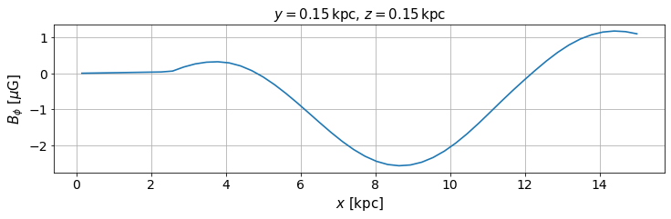
Now the galactic magnetic field has been computed and is stored in the B_field object. Specific field components can be accessed in the same way as grid components were accessed. The following snippet exemplifies this showing the \(x\)-depence of \(B_\phi\).
[5]:
x = B.grid.x[50:,50,50]
Bphi = B.phi[50:,50,50]
y = B.grid.x[50,50,50]
z = B.grid.x[50,50,50]

import galmag.analysis.visualization as visu
visu.std_setup() # Sets matplotlib's rc parameters (fonts, colors, sizes, etc)

plt.figure(figsize=(12,3))
plt.title(r'$y={0:.2f}\,\rm kpc$, $z={1:.2f}\,\rm kpc$'.format(y,z))
plt.plot(x, Bphi)
plt.xlabel(r'$x\,\,[{\rm kpc}]$')
plt.ylabel(r'$B_\phi\,\,[\mu{\rm G}]$')
plt.grid()

plt.figure(figsize=(8,7))
plt.title(r'$z={0:.2f} \,\rm kpc$'.format(z))
visu.plot_x_y_uniform(B.disk, iz=50, field_lines=False);
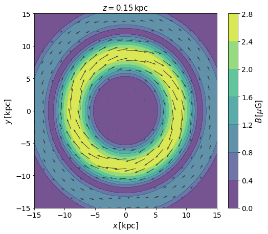
Obs. Note that the slicing used to create the previous plot exploits the fact that the indices in the cartesian follow the coordinates (i.e. the first index corresponds to \(x\), the second to \(y\) and the third to \(z\)).
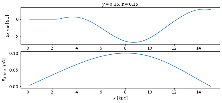
Separate field information can be accessed at any point through the attributes B_field.disk and B_field.halo. For example, it is possible to plot the \(x\)-dependence of the halo field in the following way.
[6]:
x = B.grid.x[50:,50,50]
Bphi_halo = B.halo.phi[50:,50,50]
Bphi_disk = B.disk.phi[50:,50,50]
y = B.grid.x[50,50,50]
z = B.grid.x[50,50,50]

plt.figure(figsize=(12,5))

plt.subplot(2,1,1)
plt.title('$y={0:.2f}$, $z={1:.2f}$'.format(y,z), fontsize=14)
plt.plot(x, Bphi_disk, )
plt.ylabel(r'$B_{\phi,\rm disk}\,\,[\mu{\rm G}]$', fontsize=14)

plt.subplot(2,1,2)
plt.plot(x, Bphi_halo, )
plt.xlabel(r'$x\,\,[{\rm kpc}]$', fontsize=14)
plt.ylabel(r'$B_{\phi,\rm halo}\,\,[\mu{\rm G}]$', fontsize=14);
All the used parameters can be accessed at any point through the parameters attribute, which contain a dictionary.
[7]:
B.parameters
[7]:
{'disk_modes_normalization': array([ 1.26205786,  0.20083939, -1.54587971]),
 'disk_height': 0.5,
 'disk_radius': 17.0,
 'disk_turbulent_induction': 0.386392513,
 'disk_dynamo_number': -20.4924192,
 'disk_shear_function': <function galmag.disk_profiles.Clemens_Milky_Way_shear_rate(R, R_d=1.0, Rsun=8.5, normalize=True)>,
 'disk_rotation_function': <function galmag.disk_profiles.Clemens_Milky_Way_rotation_curve(R, R_d=1.0, Rsun=8.5, normalize=True)>,
 'disk_height_function': <function galmag.disk_profiles.exponential_scale_height(R, h_d=1.0, R_HI=5, R_d=1.0, Rsun=8.5)>,
 'disk_regularization_radius': None,
 'disk_ref_r_cylindrical': 8.5,
 'disk_field_decay': True,
 'disk_newman_boundary_condition_envelope': False,
 'halo_symmetric_field': True,
 'halo_n_free_decay_modes': 4,
 'halo_dynamo_type': 'alpha2-omega',
 'halo_rotation_function': <function galmag.halo_profiles.simple_V(rho, theta, phi, r_h=1.0, Vh=220, fraction=0.2, normalize=True, fraction_z=None, legacy=False)>,
 'halo_alpha_function': <function galmag.halo_profiles.simple_alpha(rho, theta, phi, alpha0=1.0)>,
 'halo_Galerkin_ngrid': 501,
 'halo_growing_mode_only': False,
 'halo_compute_only_one_quadrant': True,
 'halo_turbulent_induction': 4.331,
 'halo_rotation_induction': 203.65472,
 'halo_radius': 15.0,
 'halo_ref_radius': 8.5,
 'halo_ref_z': 0.02,
 'halo_ref_Bphi': 0.1,
 'halo_rotation_characteristic_radius': 3.0,
 'halo_rotation_characteristic_height': 1000,
 'halo_manually_specified_coefficients': None,
 'halo_do_not_normalize': False,
 'halo_field_growth_rate': (0.002791486037391211+7.133179987229059j),
 'halo_field_coefficients': array([ 0.14206043,  0.85703689,  0.09889403, -0.41846486])}
All the parameter names can be used as keyword arguments for the methods add_disk_field and add_halo_field previously shown.
Also, it is possible (and preferable) to access separately the parameters associated with a specific component – i.e. halo or disc.
[8]:
B.disk.parameters
[8]:
{'disk_modes_normalization': array([ 1.26205786,  0.20083939, -1.54587971]),
 'disk_height': 0.5,
 'disk_radius': 17.0,
 'disk_turbulent_induction': 0.386392513,
 'disk_dynamo_number': -20.4924192,
 'disk_shear_function': <function galmag.disk_profiles.Clemens_Milky_Way_shear_rate(R, R_d=1.0, Rsun=8.5, normalize=True)>,
 'disk_rotation_function': <function galmag.disk_profiles.Clemens_Milky_Way_rotation_curve(R, R_d=1.0, Rsun=8.5, normalize=True)>,
 'disk_height_function': <function galmag.disk_profiles.exponential_scale_height(R, h_d=1.0, R_HI=5, R_d=1.0, Rsun=8.5)>,
 'disk_regularization_radius': None,
 'disk_ref_r_cylindrical': 8.5,
 'disk_field_decay': True,
 'disk_newman_boundary_condition_envelope': False}
(This is actually safer than just using ``B_field.parameters``)
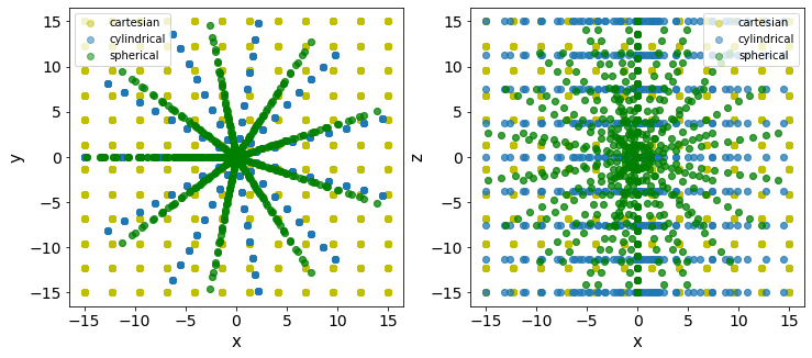
Grid object
All the calculations are done on top of a coordinate grid, which is stored as a `Grid <http://galmag.readthedocs.io/en/latest/galmag.html#galmag.Grid.Grid>`__ object. This class can be directly accessed from the module Grid, and instantiated using a similar syntax as the one used for the B_field.
[9]:
# A cartesian grid can be constructed as follows
cartesian_grid = galmag.Grid(box=[[-15, 15],[-15, 15],[-15, 15]],
                      resolution = [12,12,12],
                      grid_type = 'cartesian' # Optional
                      )
# For cylindrical grid, the limits are specified assuming
# the order: r (cylindrical), phi, z
cylindrical_grid = galmag.Grid(box=[[0.25, 15],[-np.pi,np.pi],[-15,15]],
                      resolution = [9,12,9],
                      grid_type = 'cylindrical')

# For spherical grid, the limits are specified assuming
# the order: r (spherical), theta, phi (azimuth)
spherical_grid = galmag.Grid(box=[[0, 15],[0, np.pi], [-np.pi,np.pi],],
                      resolution = [12,10,10],
                      grid_type = 'spherical')
The geometry of the different grids can be easily understood from the following plot (note the automatic conversion to cartesian coordinates through the attributes x, y, z).
[10]:
plt.figure(figsize=(12,5))
plt.subplot(1,2,1)
plt.scatter(cartesian_grid.x, cartesian_grid.y, color='y', label='cartesian', alpha=0.5)
plt.scatter(cylindrical_grid.x, cylindrical_grid.y, label='cylindrical', alpha=0.5)
plt.scatter(spherical_grid.x, spherical_grid.y, color='g', label='spherical', alpha=0.5)
plt.xlabel('x'); plt.ylabel('y')
plt.legend()

plt.subplot(1,2,2)
plt.scatter(cartesian_grid.x, cartesian_grid.z, color='y', label='cartesian', alpha=0.5)
plt.scatter(cylindrical_grid.x, cylindrical_grid.z, label='cylindrical', alpha=0.5)
plt.scatter(spherical_grid.x, spherical_grid.z, label='spherical', color='g', alpha=0.5)
plt.xlabel('x'); plt.ylabel('z')
plt.legend();
Disc field
The disc field in GalMag is constructed by expanding the dynamo solution (associated with a given choice of parameters) in a series of modes and assigning an adequate choice of coefficients \(C_n\!\)’s to the \(n\) dominant modes.
Direct choice of normalizations
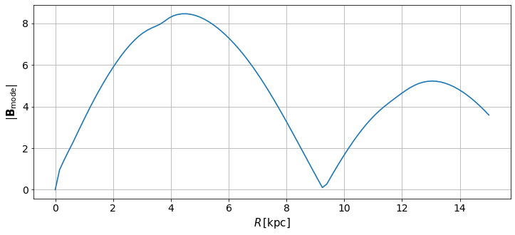
The choice of the \(C_n\)’ can be done explicitly setting up the parameter disk_modes_normalization, which should contain an array of coefficients. Each mode is pre-normalized so that its absolute value at a reference cylindrical radius is unit, i.e. \(| \mathbf{B}_{\rm mode}(R_{\rm ref},0,0)|=1\,\). \(\;R_{\rm ref}\) is set by the parameter disk_ref_r_cylindrical, whose default value is \(8.5\,{\rm kpc}\), roughly the Sun’s radius.
To exemplify this, we will generate a new B_field object based on an uniform cylindrical grid and add to it a disc magnetic field corresponding to the second mode only.
[11]:
plt.figure(figsize=(12,5))
box_limits = [[1e-8, 15],# r [kpc]
              [0,0], # phi
              [0,0]] # z [kpc]
box_resolution = [100,1,1] # No phi or z variation
Bcyl = B_field(box_limits, box_resolution, grid_type='cylindrical')

Bcyl.add_disk_field(disk_modes_normalization=[0,2]) # Skips first mode, normalization 2 for the second mode

y = np.sqrt(Bcyl.r_cylindrical[:,0,0]**2 + Bcyl.phi[:,0,0]**2 +Bcyl.z[:,0,0]**2)
x = Bcyl.grid.r_cylindrical[:,0,0]
plt.plot(x,y)
plt.ylabel(r'$| \mathbf{B}_{\rm mode}|$')
plt.xlabel(r'$R\,[{\rm kpc}]$')
plt.grid();
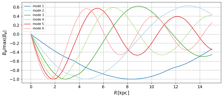
For a more interesting application, let us examine how \(B_\phi\) components of the different modes behave.
[12]:
plt.figure(figsize=(12,5))
box_limits = [[1e-8, 15],# r [kpc]
              [0,0], # phi
              [0,0]] # z [kpc]
box_resolution = [100,1,1] # No phi or z variation
Bcyl = B_field(box_limits, box_resolution, grid_type='cylindrical')

nmodes = 6

for i in range(nmodes):
    mode_norm = np.zeros((i+1))
    mode_norm[i]=1

    # Overwrites the disk field with another mode
    Bcyl.add_disk_field(disk_modes_normalization=mode_norm)

    x = Bcyl.grid.r_cylindrical[:,0,0]
    y = Bcyl.phi[:,0,0]
    plt.plot(x,y/abs(y).max(), label='mode {}'.format(i+1))
    plt.ylabel(r'$B_\phi/\max(B_\phi)$')
    plt.xlabel(r'$R\,[{\rm kpc}]$')
plt.legend(loc='upper left')
plt.grid();
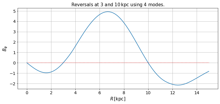
Reversals
As it was discussed in the Quick Start section, the disk field can be constructed by specifying the position of the magnetic field reversals (positions \(R_{\rm rev}\) along the mid-plane where \(B_\phi\) changes sign), the strength of the field at a reference point (generally \(R_{\rm Sun}\approx 8.5\,{\rm kpc}\)) and the number of modes to be used.
This is done using a least squares method to find the choice of \(C_n\)’s which offers best fit to these constraints. It is worth noting that such solution is not necessarily unique and, for some special cases, may not be exact.
Thus, while this is a good tool for the quick generation of examples, the user should use it carefully.
[13]:
plt.figure(figsize=(12,5))
reversals_positions = [3,10]
B_phi_ref = 3 # muG
number_of_modes = 4

Bcyl.add_disk_field(reversals=reversals_positions,
                    B_phi_ref=B_phi_ref,
                    number_of_modes=number_of_modes)

y = Bcyl.phi[:,0,0]
x = Bcyl.grid.r_cylindrical[:,0,0]
plt.title(r'Reversals at $3$ and $10\,\rm kpc$ using 4 modes.')
plt.plot(x,x*0, 'r:', alpha=0.75)
plt.plot(x,y)
plt.ylabel(r'$B_\phi$')
plt.xlabel(r'$R\,[{\rm kpc}]$')
plt.grid();
GalMag’s choice of \(C_n\)’s can found in the parameters dictionary, under the name disk_modes_normalization.
[14]:
Bcyl.parameters
[14]:
{'disk_modes_normalization': array([-0.91287645, -0.82464857,  0.83137772,  0.43987423]),
 'disk_height': 0.5,
 'disk_radius': 17.0,
 'disk_turbulent_induction': 0.386392513,
 'disk_dynamo_number': -20.4924192,
 'disk_shear_function': <function galmag.disk_profiles.Clemens_Milky_Way_shear_rate(R, R_d=1.0, Rsun=8.5, normalize=True)>,
 'disk_rotation_function': <function galmag.disk_profiles.Clemens_Milky_Way_rotation_curve(R, R_d=1.0, Rsun=8.5, normalize=True)>,
 'disk_height_function': <function galmag.disk_profiles.exponential_scale_height(R, h_d=1.0, R_HI=5, R_d=1.0, Rsun=8.5)>,
 'disk_regularization_radius': None,
 'disk_ref_r_cylindrical': 8.5,
 'disk_field_decay': True,
 'disk_newman_boundary_condition_envelope': False}
Disc parameters
The following parameters control the disc magnetic field:
disk_dynamo_number- Default: -20.49Dynamo number, \(D= R_\omega R_\alpha\), associated with the disc component.disk_field_decay- Default: TrueSets behaviour for \(|z|>h(R)\). IfTrue, the field will decay with \(|z|^{-3}\), otherwise, the field will be assumed to be constant.disk_height- Default: 0.5 \([\rm kpc ]\),Disc height at the solar radius, \(h_\odot\).disk_height_function- Default:galmag.disk_profiles.exponential_scale_heightDisc height as a function of the cylindrical radius, \(h(R)\). The default function corresponds to an exponential disc. A function of a constant height disc can be found ingalmag.disk_profiles.constant_scale_heightdisk_modes_normalization.An n-array containing the the coefficients of the first n modes (see Direct choice of normalizations section).disk_radius- Default: 17 \([\rm kpc]\)Radius of the dynamo active region of the disc.disk_rotation_function- Default:galmag.disk_profiles.Clemens_Milky_Way_rotation_curveRotation curve of the disc. By default, assumes the rotation curve obtained by Clemens (1985). One alternative, mostly for testing isgalmag.disk_profiles.solid_body_rotation_curvedisk_shear_function- Default:galmag.disk_profiles.Clemens_Milky_Way_shear_rateShear rate as a function of the cylindrical radius of the disc. By default, assumes a shear rate compatible with the rotation curve obtained by Clemens (1985). Also available is (again, mostly for testing) is a constant shear profile:galmag.disk_profiles.constant_shear_rate.disk_turbulent_induction- Default: 0.386,Dimensionless intensity of helical turbulence, \(R_\alpha\).disk_ref_r_cylindrical: 8.5 \([\rm kpc]\)Reference cylindrical radius corresponding, \(s_0\). This is used both for the normalization of the magnetic field and for the normalization of the height profile.
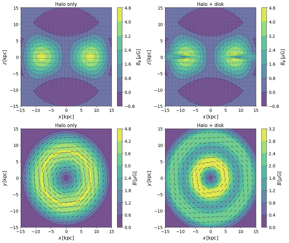
Halo field
To specify the halo field, one chooses the field strength at a reference position, whether the field is symmetric or anti-symmetric and the number of free-decay modes used to construct the solution. All these (and other parameters listed later) can be used as arguments for the B_field.add_halo_field method.
Generally, more than one solution is found for a given set of parameters. The B_field.add_halo_field method will include the one with the largest growth rate.
It is possible to access the growth/decay rate of the solution found through the attribute B_field_component.growth_rate.
Similarly, the coefficients used can be accessed using B_field_component.coefficients.
[15]:
# Using the previously defined B object
B.add_halo_field(
    # Number of free decay modes to be used in the Galerkin expansion
    halo_n_free_decay_modes = 4,
    # cylindrical radius of the reference point
    halo_ref_radius = 9,
    # z coordinate of the reference point
    halo_ref_z = 0.02,
    # B_phi value at the reference point
    halo_ref_Bphi = 4.1, # [muG]
    # Chooses between symmetric and anti-symmetric solution
    halo_symmetric_field = True # Symmetric
    )
[16]:
plt.figure(figsize=(13.1,11))
plt.subplot(2,2,1)
plt.title('Halo only')
visu.plot_x_z_uniform(B.halo, skipx=4,skipz=4, iy=49)
plt.subplot(2,2,2)
plt.title('Halo + disk')
visu.plot_x_z_uniform(B, skipx=4,skipz=4, iy=49)
plt.subplot(2,2,3)
plt.title('Halo only')
visu.plot_x_y_uniform(B.halo, skipy=5,skipx=5, iz=49, field_lines=False)
plt.subplot(2,2,4)
plt.title('Halo + disk')
visu.plot_x_y_uniform(B, skipy=5,skipx=5, iz=49, field_lines=False)
plt.tight_layout()
[17]:
print('Growth rate: ', B.halo.growth_rate)
print('Coefficients: ', B.halo.coefficients)
B.halo.parameters
Growth rate:  (0.002791486037391211+7.133179987229059j)
Coefficients:  [ 0.14206043  0.85703689  0.09889403 -0.41846486]
[17]:
{'halo_symmetric_field': True,
 'halo_n_free_decay_modes': 4,
 'halo_dynamo_type': 'alpha2-omega',
 'halo_rotation_function': <function galmag.halo_profiles.simple_V(rho, theta, phi, r_h=1.0, Vh=220, fraction=0.2, normalize=True, fraction_z=None, legacy=False)>,
 'halo_alpha_function': <function galmag.halo_profiles.simple_alpha(rho, theta, phi, alpha0=1.0)>,
 'halo_Galerkin_ngrid': 501,
 'halo_growing_mode_only': False,
 'halo_compute_only_one_quadrant': True,
 'halo_turbulent_induction': 4.331,
 'halo_rotation_induction': 203.65472,
 'halo_radius': 15.0,
 'halo_ref_radius': 9,
 'halo_ref_z': 0.02,
 'halo_ref_Bphi': 4.1,
 'halo_rotation_characteristic_radius': 3.0,
 'halo_rotation_characteristic_height': 1000,
 'halo_manually_specified_coefficients': None,
 'halo_do_not_normalize': False,
 'halo_field_growth_rate': (0.002791486037391211+7.133179987229059j),
 'halo_field_coefficients': array([ 0.14206043,  0.85703689,  0.09889403, -0.41846486])}
Galerkin expansion coefficients
It is likely that one may want to study directly which choices of parameters lead to which growth rates. This can be done using the module galmag.galerkin, which contains the function Galerkin_expansion_coefficients.
[18]:
from galmag.galerkin import Galerkin_expansion_coefficients
The function requires a dictionary containing the following parameters (described individually in the comments):
[19]:
p = { # Square root of the number of grid points used in the calculations
      'halo_Galerkin_ngrid': 500,
      # Function specifying the alpha profile of the halo
      'halo_alpha_function': galmag.halo_profiles.simple_alpha,
      # R_\alpha
      'halo_turbulent_induction': 7.7,
      # R_\omega
     'halo_rotation_induction': 200.0,
      # Number of free decay modes to be used for the expansion
     'halo_n_free_decay_modes': 4,
      # Whether the field is symmetric or antisymmetric
      'halo_symmetric_field': True,
      # Defines the dynamo type
      'halo_dynamo_type': 'alpha-omega',
      # Function specifying the rotation curve of the halo
      'halo_rotation_function': galmag.halo_profiles.simple_V,
      # Parameters used in this function
      'halo_rotation_characteristic_height': 1e3,
      'halo_rotation_characteristic_radius': 3.0,
      # Halo radius
      'halo_radius': 20.,
     }
The function returns the growth rates and the coefficients, \(a_i\) of the free decay modes. Optionally, the intermediate matrix \(W_{ij} = \int \mathbf{B_j} \cdot \hat{W} \,\mathbf{B_i} \;{\rm d}^3\mathbf{r}\;\) is
[20]:
vals, vecs, Wij = Galerkin_expansion_coefficients(p, return_matrix=True)
[21]:
print('The resultant matrix is:\n', Wij)

for i, (val, vec) in enumerate(zip(vals, vecs)):
    print('\nSolution ',i)
    print(' Growth rate =', val)
    for i, c in enumerate(vec):
        print('    a{0} = {1}'.format(i+1, c))
The resultant matrix is:
 [[-2.01907286e+01  1.25802759e+01  1.98763272e+01  1.49637059e+01]
 [ 1.38178883e+02 -2.01907286e+01 -1.12133344e+01  0.00000000e+00]
 [-7.44585112e+00  1.11181174e-03 -4.88311936e+01 -2.27594189e+01]
 [-7.28554698e+01  0.00000000e+00 -1.54579219e+02 -4.88311936e+01]]

Solution  0
 Growth rate = (-82.5472249922034+9.72793002473695j)
    a1 = (-0.3304728627932634+0.04590311536614698j)
    a2 = (-0.3304728627932634-0.04590311536614698j)
    a3 = (0.19556281135575382+0.039281681425336674j)
    a4 = (0.19556281135575382-0.039281681425336674j)

Solution  1
 Growth rate = (-82.5472249922034-9.72793002473695j)
    a1 = (0.7728996311795923+0j)
    a2 = (0.7728996311795923-0j)
    a3 = (0.7782745573919754+0j)
    a4 = (0.7782745573919754-0j)

Solution  2
 Growth rate = (13.525302792151383+9.587979337319839j)
    a1 = (0.2257082569733093-0.10486375376800403j)
    a2 = (0.2257082569733093+0.10486375376800403j)
    a3 = (0.06976706192021101-0.18140737243306812j)
    a4 = (0.06976706192021101+0.18140737243306812j)

Solution  3
 Growth rate = (13.525302792151383-9.587979337319839j)
    a1 = (0.39769866232974604-0.26683684329612717j)
    a2 = (0.39769866232974604+0.26683684329612717j)
    a3 = (-0.3315122408562829+0.45477951371599235j)
    a4 = (-0.3315122408562829-0.45477951371599235j)
Halo parameters
halo_Galerkin_ngridNumber of grid points used for the Galerkin expansion calculations.halo_alpha_function- Default:galmag.halo_profiles.simple_alphaalpha-effect profile. By default, it is assumed simply: \(\alpha \propto \cos(\theta)\,\).halo_dynamo_type- Default:'alpha2-omega'Chooses the dominant type of dynamo. Available options:'alpha-omega'and'alpha2-omega'.halo_growing_mode_only- Default:False.If true, returns a zero field if all modes are decaying for a particular choice of parameters.halo_n_free_decay_modes- Default:4Number of free decay modes to be used for the Galerkin expansion.halo_radius- Default: 15 [\({\rm kpc}\)]Radius of the dynamo active region of the halo.halo_ref_Bphi- Default: -0.5 [\({\mu\rm G}\)]Strength of the halo magnetic field at the halo reference point.halo_ref_radius- Default: 8.5 [\({\rm kpc}\)]Cylindrical radius of the halo reference point.halo_ref_z- Default: 0.02 [\({\rm kpc}\)]z-coordinate of the halo reference point.halo_rotation_function- Default:galmag.halo_profiles.simple_VRotation curve of the halo. By default a simple rotation curve with no z dependence, exponentially decaying with the cylindrical radius, is assumed.halo_rotation_induction- Default: 203.65Dimensionless induction by differential rotation, \(R_\omega\), for the halo.halo_symmetric_field- Default:TrueIf True, the field is assumed to be symmetric over the midplane. If False, it is assumed to be anti-symmetric.halo_turbulent_induction: 4.331Dimensionless intensity of helical turbulence, \(R_\alpha\), for the halo.
Plotting tools
GalMag comes with a small selection of plotting tools, particularly to facilitate the preparation of 2D slices for diagnostic. These can be found in the galmag.analysis.visualization module.
[22]:
help(galmag.analysis.visualization)
Help on module galmag.analysis.visualization in galmag.analysis:

NAME
    galmag.analysis.visualization

FUNCTIONS
    plot_r_z_uniform(B, skipr=3, skipz=5, quiver=True, contour=True, quiver_color='0.25', cmap='viridis', field_lines=True, vmin=None, vmax=None, levels=None, **kwargs)
        Plots a r-z slice of the field. Assumes B is created using a cylindrical
        grid - for a more sophisticated/flexible plotting script which does not
        rely on the grid structure check the plot_slice.

        The plot consists of:
          1) a coloured contourplot of :math:`B_\phi`
          2) quivers showing the x-z projection of the field

        Parameters
        ----------
        B : B_field
            a B_field or B_field_component object
        quiver : bool
            If True, shows quivers. Default True
        contour : bool
            If True, shows contours. Default: True
        skipx/skipz : int
            Tweaks the display of quivers (Default: skipz=5, skipr=3)

    plot_slice()
        Plots slice of arbitrary orientation

        Note
        ----
        Not implemented yet

    plot_x_y_uniform(B, skipx=5, skipy=5, iz=0, field_lines=True, quiver=True, vmin=None, vmax=None, contour=True, levels=None, quiver_color='0.25', cmap='viridis', **kwargs)
        Plots a x-y slice of the field. Assumes B is created using a cartesian
        grid - for a more sophisticated/flexible plotting script which does not
        rely on the grid structure check the plot_slice.

        The plot consists of:
          1) a coloured contourplot of :math:`|B|^2`
          2) Field lines of the :math:`B_x` and :math:`B_y` field
          3) Quivers showing the :math:`B_x` and :math:`B_y` field

        Parameters
        ----------
        B : B_field
            a B_field or B_field_component object
        field_lines : bool
            If True, shows field lines. Default: True
        quiver : bool
            If True, shows quivers. Default True
        contour : bool
            If True, shows contours. Default: True
        skipx/skipy : int
            Tweaks the display of quivers (Default: skipx=5, skipy=5)

    plot_x_z_uniform(B, skipx=1, skipz=5, iy=0, quiver=True, contour=True, quiver_color='0.25', cmap='viridis', vmin=None, vmax=None, no_colorbar=False, **kwargs)
        Plots a x-z slice of the field. Assumes B is created using a cartesian
        grid - for a more sophisticated/flexible plotting script which does not
        rely on the grid structure check the plot_slice.

        The plot consists of:
          1) a coloured contourplot of :math:`B_\phi`
          2) quivers showing the x-z projection of the field

        Parameters
        ----------
        B : B_field
            a B_field or B_field_component object
        quiver : bool
            If True, shows quivers. Default True
        contour : bool
            If True, shows contours. Default: True
        skipx/skipz : int
            Tweaks the display of quivers (Default: skipz=5, skipx=1)

    plot_y_z_uniform(B, skipy=5, skipz=5, ix=0, quiver=True, contour=True, quiver_color='0.25', cmap='viridis', vmin=None, vmax=None, **kwargs)
        Plots a y-z slice of the field. Assumes B is created using a cartesian
        grid - for a more sophisticated/flexible plotting script which does not
        rely on the grid structure check the plot_slice.

        The plot consists of:
          1) a coloured contourplot of :math:`B_\phi`
          2) Quivers showing the y-z projection of the field

        Parameters
        ----------
        B : B_field
            a B_field or B_field_component object
        quiver : bool
            If True, shows quivers. Default True
        contour : bool
            If True, shows contours. Default: True
        skipy/skipz : int
            Tweaks the display of quivers (Default: skipz=5, skipy=5)

    std_setup()
        Adjusts matplotlib default settings

FILE
    /home/lrodrigues/GalMag/galmag/analysis/visualization.py
Advanced
Adding extra major components: Gaussian random field example
If one explores the B_field object a little further, one finds there is a method called B_field.set_field_component which takes a component name and a B_field_component object as inputs.
We exemplify, below, how to add an extra personalised Gaussian random field component to our B_field object.
We start by generating the noisy field. To keep things divergence-free we first construct a random vector potential, \(\mathbf A\), and then take the curl of it.
[23]:
from galmag.util import derive

mu = 0
sigma = 0.0778 # magic number to generate Brms~0.5
print(sigma)
# Defines a random vector potential
A_rnd = {} # Dictionary of vector components
for i, c in enumerate(('x','y','z')):
    A_rnd[c] = np.random.normal(mu, sigma, B.resolution.prod())
    A_rnd[c] = A_rnd[c].reshape(B.resolution)

# Prepares the derivatives to compute the curl
dBi_dj ={}
for i, c in enumerate(['x','y','z']):
    for j, d in enumerate(['x','y','z']):
        dj = (B.box[j,-1]-B.box[j,0])/float(B.resolution[j])
        dBi_dj[c,d] = derive(A_rnd[c],dj, axis=j)

# Computes the curl of A_rnd
tmpBrnd = {}
tmpBrnd['x'] = dBi_dj['z','y'] -  dBi_dj['y','z']
tmpBrnd['y'] = dBi_dj['x','z'] -  dBi_dj['z','x']
tmpBrnd['z'] = dBi_dj['y','x'] -  dBi_dj['x','y']

del dBi_dj; del A_rnd

for c in tmpBrnd:
    print('B{0}: mean = {1}  std = {2}'.format(c,
                                                tmpBrnd[c].mean(),
                                                tmpBrnd[c].std()))
0.0778
Bx: mean = -0.00017563838972479574  std = 0.288666276254484
By: mean = 0.0001620638666346189  std = 0.2886417232520821
Bz: mean = 5.918382704113669e-05  std = 0.2882613118574375
Note that the format is compatible with the grid of the previously generated field object.
Now, we can use these data create a B_field_component object. Note that we included the parameters used for generating the data for future reference.
[24]:
from galmag.B_field import B_field_component
Brnd_component = B_field_component(B.grid,
                                     x=tmpBrnd['x'],
                                     y=tmpBrnd['y'],
                                     z=tmpBrnd['z'],
                                     parameters={'mu': mu,
                                                 'sigma':sigma})
del tmpBrnd
One can now access the x,y,z vector components through the Brnd_component’s attributes.
One can also access the same information in a cylindrical or spherical coordinate system.
[25]:
print('A sample of Brnd_x')
print(Brnd_component.x[1:3,1:3,1:3])
print('\nA sample of Brnd_theta')
print(Brnd_component.theta[1:3,1:3,1:3])
A sample of Brnd_x
[[[-0.11884636 -0.11828462]
  [ 0.32860367 -0.43862623]]

 [[-0.15642111 -0.34380286]
  [-0.0559142   0.37455865]]]

A sample of Brnd_theta
[[[ 0.00549858  0.0563936 ]
  [ 0.48793848 -0.00555552]]

 [[-0.65227692  0.31251592]
  [-0.06968609  0.14013689]]]
Finally, one can add this component to the previously defined B_field object using
[26]:
B.set_field_component('random',Brnd_component)

print('Brms', (B.random.x**2+B.random.y**2+B.random.z**2).mean()**0.5)
Brms 0.4997368387247418
Now the new component can be accessed easily using B.random.
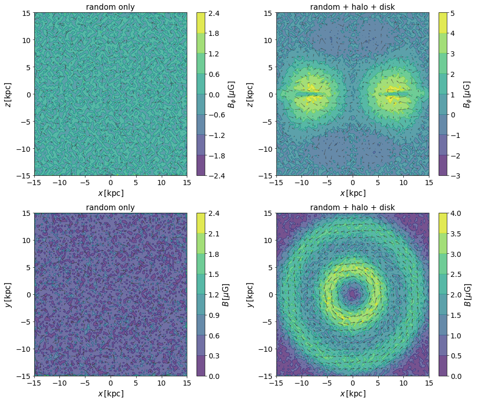
[27]:
plt.figure(figsize=(13.1,11))
plt.subplot(2,2,1)
plt.title('random only')
visu.plot_x_z_uniform(B.random, skipx=4,skipz=4, iy=49)

plt.subplot(2,2,2)
plt.title('random + halo + disk')
visu.plot_x_z_uniform(B, skipx=4,skipz=4, iy=49)

plt.subplot(2,2,3)
plt.title('random only')
visu.plot_x_y_uniform(B.random, skipy=4,skipx=4, iz=49, field_lines=False)

plt.subplot(2,2,4)
plt.title('random + halo + disk')
visu.plot_x_y_uniform(B, skipy=4,skipx=4, iz=49, field_lines=False)
plt.tight_layout()
Generators
To produce the built-in field and halo field components, a generator class is used. The generator is actually stored in the B_component_field object itself. E.g.
[28]:
B.halo.generator?
Type:        B_generator_halo
String form: <galmag.B_generators.B_generator_halo.B_generator_halo object at 0x7fd8dbdb6090>
File:        ~/GalMag/galmag/B_generators/B_generator_halo.py
Docstring:
Generator for the halo field

Parameters
----------
box : 3x2-array_like
     Box limits
resolution : 3-array_like
     containing the resolution along each axis.
grid_type : str, optional
    Choice between 'cartesian', 'spherical' and 'cylindrical' *uniform*
    coordinate grids. Default: 'cartesian'
dtype : numpy.dtype, optional
    Data type used. Default: np.dtype(np.float)
Most of the physics is coded in the generator classes \(-\) while the B_field and B_field_component classes deal only with coordinate transformations and convenience.
galmag.B_generators.B_generator_halo.B_generator_halo and galmag.B_generators.B_generator_disk.B_generator_disk for further details on the computation of the magnetic fields.One can use the generators directly to produce the magnetic field components (and then possibly include them using the set_field_component method). Also, for the sake of consistency, long term inclusion of new components (e.g. a random/turbulent field component) should be implemented using similar generators.